Sound Data Stories

PSRC now has OMX-format trip tables available for public use. Trip tables are two-dimensional matrices containing the estimated number of trips between any two origin/destination points in the Puget Sound region. The tables for our region are aggregated into 3,700 neighborhoods (or “zones”) for convenience, so the matrices are 3700x3700 in size. You can think of a trip table as a big “from/to” table, on a neighborhood-to-neighborhood scale.

Download the file here: PSRC 2010 OMX Trip Tables

Trips are stored separately by:

• Mode (auto, transit, bike, walk, etc)
• Household income quartile, for work trips
• Time period (A.M. peak, midday, P.M. peak, evening, late-night)

How were these tables created?

We use the PSRC travel model to predict the travel patterns of area residents. The model is based on census data, local survey data, and human behavior research to produce a reasonable estimate of travel patterns. These are just estimates and can’t possibly predict or capture every nuance of human behavior, but they’re useful for analyzing the effects of growth and investment in our transportation infrastructure.

How do I look at these?

The OMX format is an open format jointly created by PSRC and several other public and private agencies in the transportation planning field. It was expressly designed to allow sharing of matrix data amongst planning agencies and with the public. You can download the OMX Viewer app for Windows; other platforms should search for “vitables”. OMX is really just an HDF5 file with a specific layout; HDF5 can be read by pandas and pytables easily.

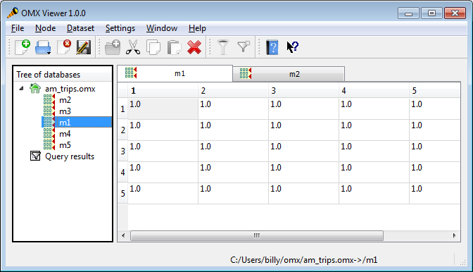The free OMX Viewer lets you browse the tables inside an OMX file. Source: OMX website

Zone definitions

You’ll also need to know the lookups for the zone numbers. The trip tables are divided into “zones” of various sizes (smaller zones in dense areas, larger in more suburban and rural areas). Zones are numbered continuously from 1-3700. Thus, to make heads or tails of these trip tables you’ll need to know what areas those numbers correspond to.

The attached zone “shape file” defines the zones. You can view this shape file using the freely available QGis program, or you can use ArcGIS if you have access to that non-free program.

To view the zone definitions boundaries and their corresponding zone numbers using the QGis application:

• Download and unzip the TAZ2010 shapefile (a “shapefile” is actually a collection of related files which define the boundaries). Be sure to unzip it after downloading.
• Open QGis and choose menu “Layer > Add Vector Layer…”, and browse/open the taz2010.shp file
• In the “Layers” panel on the left, click on the taz2010 layer to activate it
• Choose menu “Layer > Labeling”, and select “Label this layer with” and choose “TAZ”.

You can now see the zone numbers. QGis is a very advanced and feature-rich application, which is a nice way of saying it’s hard to use. It may take you a while to learn your way around it. Pro-tip: your mouse wheel will zoom the map in and out; press and hold your mouse wheel down, and then drag to pan the map.

QGis showing zone numbers, highlighting zone 553 on Seattle's Capitol Hill. Source: QGis homepage

Usage example: bike trips from Ballard

If you’re savvy with GIS, mapping the data in these trip tables is fairly straightforward. Here’s a python code snippet that uses the omx libraries (see above) to fetch the estimated midday bike trips from zone 242 (in Ballard) to all destinations. Sample python code:

import omx,numpy
trips = omx.openFile('non_motorized.omx')
midday_bikes = trips['mbike']
ballard = midday_bikes[242,:]
numpy.savetxt("ballard.csv", ballard)

Once you have that row of data, you can use GIS to map it. Here’s what such a map might look like: lots of trips to downtown, plenty around north Seattle, and a few outliers further afield:

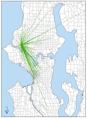2010 estimated bike trips from Ballard (zone 242) Source: PSRC travel model

What next?

We’re excited to finally be able to provide this data to you in an open format, and are curious to see what you do with it. You could pull one column from a trip table to get all the morning commute trips into a block of downtown Seattle, for example. Or pull a row for your home zone to see the travel destinations of all the households in your neighborhood.

If you know the Python programming language, go back to the OMX website to see if you can crack into these OMX files and start poking around the tables yourself.

If you don’t know Python, well… we’ll be adding further blog posts soon with some recipes of how to do some of that stuff.