Combining DataFrames with pandas
In many “real world” situations, the data that we want to use come in multiple files. We often need to combine these files into a single DataFrame to analyze the data. The pandas package provides various methods for combining DataFrames.
Learning Objectives
- Learn how to join two DataFrames together using a uniqueID found in both DataFrames
- Learn how to write out a DataFrame to csv using Pandas
- Learn how to clean up notebooks and create scripts
Joining DataFrames
If we look back at the surveys_df, we have an unhelpful 2-letter abbreviation for city. Our friends have given us a nice lookup table for the real city name, plus the county and a housing district they use to quantify results. They’ve asked us to clean up the early results so they can see results with the full city name. They’ve also asked that we give them information on low income households in King County.
To work through the examples below, we first need to load the housing_zone and surveys files into pandas DataFrames. In iPython:
import pandas as pd
surveys_df = pd.read_csv("surveys.csv")

city_df = pd.read_csv('city.csv')
For example, the city.csv file that we’ve been working with is a lookup
table. This table contains the city_name, housing_zone and county code for most cities in the region. The
housing_zone code is unique for each line. The city is identified in our survey
data as well using the unique city code. Rather than adding 3 more columns
for the city_name, housing_zone and county to each of the 35,549 line Survey data table, we
can maintain the shorter table with the housing_zone information. When we want to
access that information, we can create a query that joins the additional columns
of information to the Survey data.
Storing data in this way has many benefits including:
- It ensures consistency in the spelling of city attributes (
city_name,housing_zone, and county) given eachhousing_zoneis only entered once. Imagine the possibilities for spelling errors when entering thecity_nameandhousing_zonethousands of times! - It also makes it easy for us to make changes to the housing_zone information once without having to find each instance of it in the larger survey data.
- It optimizes the size of our data.
Identifying join keys
To identify appropriate join keys we first need to know which field(s) are shared between the files (DataFrames). We might inspect both DataFrames to identify these columns. If we are lucky, both DataFrames will have columns with the same name that also contain the same data. If we are less lucky, we need to identify a (differently-named) column in each DataFrame that contains the same information.
city.columns

Index([u'city', u'city_name', u'species', u'county'], dtype='object')

survey.columns

Index([u'record_id', u'month', u'day', u'year', u'district', u'city',
       u'tenure', u'hindfoot_length', u'income'], dtype='object')
In our example, the join key is the column containing the two-letter species
identifier, which is called city.
Now that we know the fields with the common housing_zone ID attributes in each DataFrame, we are almost ready to join our data. However, since there are different types of joins, we also need to decide which type of join makes sense for our analysis.
Inner joins
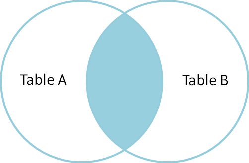
The most common type of join is called an inner join. An inner join combines two DataFrames based on a join key and returns a new DataFrame that contains only those rows that have matching values in both of the original DataFrames.
Inner joins yield a DataFrame that contains only rows where the value being joins exists in BOTH tables. An example of an inner join, adapted from this page is below:
The pandas function for performing joins is called merge and an Inner join is
the default option:
merged_inner = pd.merge(left=survey,right=city, left_on='city', right_on='city')
# in this case `city` is the only column name in  both dataframes, so if we skippd `left_on`
# and `right_on` arguments we would still get the same result

# what's the size of the output data?
merged_inner.shape
merged_inner
OUTPUT:
   record_id  month  day  year  district city tenure  hindfoot_length  \
0          1      7   16  1977        2         NL   M               32
1          2      7   16  1977        3         NL   M               33
2          3      7   16  1977        2         DM   F               37
3          4      7   16  1977        7         DM   M               36
4          5      7   16  1977        3         DM   M               35
5          8      7   16  1977        1         DM   M               37
6          9      7   16  1977        1         DM   F               34
7          7      7   16  1977        2         PE   F              NaN

   income       city_name   housing_zone   county
0     NaN     Neotoma  albigula  Rodent
1     NaN     Neotoma  albigula  Rodent
2     NaN   Dipodomys  merriami  Rodent
3     NaN   Dipodomys  merriami  Rodent
4     NaN   Dipodomys  merriami  Rodent
5     NaN   Dipodomys  merriami  Rodent
6     NaN   Dipodomys  merriami  Rodent
7     NaN  Peromyscus  eremicus  Rodent
The result of an inner join of survey and city is a new DataFrame
that contains the combined set of columns from survey and city. It
only contains rows that have two-letter housing_zone codes that are the same in
both the survey and city DataFrames. In other words, if a row in
survey has a value of city that does not appear in the city
column of cities.csv, it will not be included in the DataFrame returned by an
inner join. Similarly, if a row in city has a value of city
that does not appear in the city column of survey, that row will not
be included in the DataFrame returned by an inner join.
The two DataFrames that we want to join are passed to the merge function using
the left and right argument. The left_on='city' argument tells merge
to use the city column as the join key from survey (the left
DataFrame). Similarly , the right_on='city' argument tells merge to
use the city column as the join key from city (the right
DataFrame). For inner joins, the order of the left and right arguments does
not matter.
The result merged_inner DataFrame contains all of the columns from survey
(record id, month, day, etc.) as well as all the columns from city
(city, city_name, species, and county).
Notice that merged_inner has fewer rows than survey. This is an
indication that there were rows in surveys_df with value(s) for city that
do not exist as value(s) for city in city_df.
Left joins
What if we want to add information from city to survey without
losing any of the information from survey? In this case, we use a different
type of join called a “left outer join”, or a “left join”.
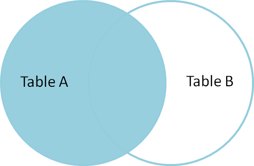
Like an inner join, a left join uses join keys to combine two DataFrames. Unlike
an inner join, a left join will return all of the rows from the left
DataFrame, even those rows whose join key(s) do not have values in the right
DataFrame. Rows in the left DataFrame that are missing values for the join
key(s) in the right DataFrame will simply have null (i.e., NaN or None) values
for those columns in the resulting joined DataFrame.
Note: a left join will still discard rows from the right DataFrame that do not
have values for the join key(s) in the left DataFrame.
A left join is performed in pandas by calling the same merge function used for
inner join, but using the how='left' argument:
merged_left = pd.merge(left=survey,right=city, how='left', left_on='city', right_on='city')

merged_left

**OUTPUT:**

   record_id  month  day  year  district city tenure  hindfoot_length  \
0          1      7   16  1977        2         NL   M               32
1          2      7   16  1977        3         NL   M               33
2          3      7   16  1977        2         DM   F               37
3          4      7   16  1977        7         DM   M               36
4          5      7   16  1977        3         DM   M               35
5          6      7   16  1977        1         PF   M               14
6          7      7   16  1977        2         PE   F              NaN
7          8      7   16  1977        1         DM   M               37
8          9      7   16  1977        1         DM   F               34
9         10      7   16  1977        6         PF   F               20

   income       city_name   housing_zone   county
0     NaN     Neotoma  albigula  Rodent
1     NaN     Neotoma  albigula  Rodent
2     NaN   Dipodomys  merriami  Rodent
3     NaN   Dipodomys  merriami  Rodent
4     NaN   Dipodomys  merriami  Rodent
5     NaN         NaN       NaN     NaN
6     NaN  Peromyscus  eremicus  Rodent
7     NaN   Dipodomys  merriami  Rodent
8     NaN   Dipodomys  merriami  Rodent
9     NaN         NaN       NaN     NaN
The result DataFrame from a left join (merged_left) looks very much like the
result DataFrame from an inner join (merged_inner) in terms of the columns it
contains. However, unlike merged_inner, merged_left contains the same
number of rows as the original survey DataFrame. When we inspect
merged_left, we find there are rows where the information that should have
come from city (i.e., city, city_name, and county) is
missing (they contain NaN values):
merged_left[ pd.isnull(merged_left.city_name) ]
**OUTPUT:**
   record_id  month  day  year  district city tenure  hindfoot_length  \
5          6      7   16  1977        1         PF   M               14
9         10      7   16  1977        6         PF   F               20

   income city_name housing_zone county
5     NaN   NaN     NaN  NaN
9     NaN   NaN     NaN  NaN
These rows are the ones where the value of city from survey (in this
case, PF) does not occur in city.
Other join types
The pandas merge function supports two other join types:
- Right (outer) join: Invoked by passing
how='right'as an argument. Similar to a left join, except all rows from therightDataFrame are kept, while rows from theleftDataFrame without matching join key(s) values are discarded. - Full (outer) join: Invoked by passing
how='outer'as an argument. This join type returns the all pairwise combinations of rows from both DataFrames; i.e., the result DataFrame willNaNwhere data is missing in one of the dataframes. This join type is very rarely used.
Final Challenges
Challenge 1
Using the filters we learned earlier, show the yearly average income for low income households in king county.
In steps:
# select all king county records
king_county_records = merged_inner[merged_inner['county'] == 'King']

# select low income records from king county dataframe
low_inc_kc = king_county_records[king_county_records['income'] < 20]

low_inc_kc.groupby('year').mean()['income'].plot(kind='bar')
Challenge 2 (together)
Move your code to complete the above challenge to a separate script.
Results are as follows:
 import pandas as pd

# Load in survey data
surveys_df = pd.read_csv('surveys.csv')

# Load in city lookup
city_df = pd.read_csv('city.csv')

# Merge survey and city file
merged_inner = pd.merge(left=surveys_df, right=city_df, left_on='city', right_on='city')

# select all low income household from king county (under 20k per year)
# show the average income over year

# select all king county records
king_county_records = merged_inner[merged_inner['county'] == 'King']

# select low income records from king county dataframe
low_inc_kc = king_county_records[king_county_records['income'] < 20]

# add a nice print statement
print 'script almost complete, writing to file'

# Write results to CSV
low_inc_kc.to_csv('my_file.csv')

print 'script done!'
If there is time for some reason, add figure creation to the script
ax = low_inc_kc.groupby('year').mean()['income'].plot(kind='bar')
fig = ax.get_figure()
fig.savefig('yearly_income_kc_low_inc.png')