R Fundamentals I
Introduction to R and RStudio
Motivation
R was designed by Ross Ihaka and Robert Gentleman in the 90’s at the University of Auckland.

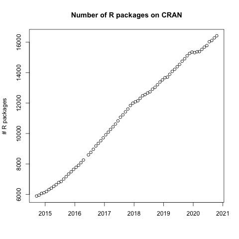
Since then R increased on popularity enormously. Currently R has several million users.
Three most widely used applications in R (from RStudio survey 2018):
- Statistical analysis (88%)
- Visualization (85%)
- Data transformation (78%)
Introduction to RStudio
We’ll be using RStudio: a free, open source R integrated development environment.
If you haven’t done so already, download and install RStudio Desktop.
It provides a built in editor, works on all platforms (including on servers) and provides many advantages such as integration with version control and project management.
Basic layout
When you first open RStudio, you will be greeted by three panels:
- The interactive R console (entire left)
- Workspace/History (tabbed in upper right)
- Files/Plots/Packages/Help (tabbed in lower right)
Once you open files, such as R scripts, an editor panel will also open in the top left.
Work flow within RStudio
There are two main ways one can work within RStudio.
- Test and play within the interactive R console then copy code into a .R file to run later.
- This works well when doing small tests and initially starting off.
- It quickly becomes laborious
- Start writing in an .R file and use RStudio’s command / short cut to push current line, selected lines or modified lines to the interactive R console.
- This is a great way to start; all your code is saved for later
- You will be able to run the file you create from within RStudio or using R’s
source()function.
R interactive console
Much of your time in R will be spent in the R interactive console. This is where you will run all of your code, and can be a useful environment to try out ideas before adding them to an R script file. This console in RStudio is the same as the one you would get if you just typed in R in your commandline environment.
The first thing you will see in the R interactive session is a bunch of information, followed by a “>” and a blinking cursor. It operates on the idea of a “Read, evaluate, print loop”: you type in commands, R tries to execute them, and then returns a result.
Introduction to R
Using R as a calculator
The simplest thing you could do with R is do arithmetic:
[1] 101
R will print out the answer, with a preceding “[1]”. Don’t worry about this for now, we’ll explain that later. For now think of it as indicating ouput.
If you type in an incomplete command, R will wait for you to complete it:
+Any time you hit return and the R session shows a “+” instead of a “>”, it means it’s waiting for you to complete the command. If you want to cancel a command you can simply hit “Esc” and RStudio will give you back the “>” prompt.
When using R as a calculator, the order of operations is the same as you would have learnt back in school.
From highest to lowest precedence:
- Parentheses:
(,) - Exponents:
^or** - Divide:
/ - Multiply:
* - Add:
+ - Subtract:
-
[1] 13
Use parentheses to group operations in order to force the order of evaluation if it differs from the default, or to make clear what you intend.
[1] 16
This can get unwieldy when not needed, but clarifies your intentions. Remember that others may later read your code.
(3 + (5 * (2 ^ 2))) # hard to read
3 + 5 * 2 ^ 2       # clear, if you remember the rules
3 + 5 * (2 ^ 2)     # if you forget some rules, this might help
The text after each line of code is called a “comment”. Anything that follows after the hash (or octothorpe) symbol # is ignored by R when it executes code.
Really small or large numbers get a scientific notation:
[1] 2e-04
Which is shorthand for “multiplied by 10^XX”. So 2e-4 is shorthand for 2 * 10^(-4).
You can write numbers in scientific notation too:
[1] 5000
Mathematical functions
R has many built in mathematical functions. To call a function, we simply type its name, followed by open and closing parentheses. Anything we type inside the parentheses is called the function’s arguments:
[1] 0.841471
[1] 0
[1] 1
[1] 1.648721
Don’t worry about trying to remember every function in R. You can simply look them up on google, or if you can remember the start of the function’s name, use the tab completion in RStudio.
This is one advantage that RStudio has over R on its own, it has autocompletion abilities that allow you to more easily look up functions, their arguments, and the values that they take.
Typing a ? before the name of a command will open the help page for that command. As well as providing a detailed description of the command and how it works, scrolling ot the bottom of the help page will usually show a collection of code examples which illustrate command usage. We’ll go through an example later.
Comparing things
We can also do comparison in R:
[1] TRUE
[1] TRUE
[1] TRUE
[1] TRUE
[1] TRUE
[1] TRUE
Variables and assignment
We can store values in variables using the assignment operator <-, like this:
Notice that assignment does not print a value. Instead, we stored it for later in something called a variable. x now contains the value 0.025:
[1] 0.025
More precisely, the stored value is a decimal approximation of this fraction called a floating point number.
Look for the Environment tab in one of the panes of RStudio, and you will see that x and its value have appeared. Our variable x can be used in place of a number in any calculation that expects a number:
[1] -3.688879
Notice also that variables can be reassigned:
x used to contain the value 0.025 and and now it has the value 100.
Assignment values can contain the variable being assigned to:
The right hand side of the assignment can be any valid R expression. The right hand side is fully evaluated before the assignment occurs.
Variable names can contain letters, numbers, underscores and periods. They cannot start with a number nor contain spaces at all. Different people use different conventions for long variable names, these include
- periods.between.words
- underscores_between_words
- camelCaseToSeparateWords
What you use is up to you, but be consistent.
Vectorization
One final thing to be aware of is that R is vectorized, meaning that variables and functions can have vectors as values. For example
[1] 1 2 3 4 5
[1] 2 4 8 16 32
[1] 2 4 8 16 32
This is incredibly powerful; we will discuss this further in an upcoming lesson.
Managing your environment
There are a few useful commands you can use to interact with the R session.
ls will list all of the variables and functions stored in the global environment (your working R session):
[1] "hook_error" "hook_in" "hook_out" "x"
Note here that we didn’t given any arguments to ls, but we still needed to give the parentheses to tell R to call the function.
You can use rm to delete objects you no longer need:
If you have lots of things in your environment and want to delete all of them, you can pass the results of ls to the rm function:
In this case we’ve combined the two. Just like the order of operations, anything inside the innermost parentheses is evaluated first, and so on.
In this case we’ve specified that the results of ls should be used for the list argument in rm. When assigning values to arguments by name, you must use the = operator!!
Reading Help files
R, and every package, provide help files for functions. To search for help on a function from a specific function that is in a package loaded into your namespace (your interactive R session):
This will load up a help page in RStudio (or as plain text in R by itself).
To seek help on special operators, use quotes:
If you’re not sure how it’s specifically spelled you can do a fuzzy search: