R Fundamentals II

More plots and writing data

Boxplot

Let’s bring in a dataset with multiple land use indicators from 2050, and merge it with city names:

lu <- read.csv(file="data/indicators2050.csv")
lu <- merge(lu, cities, by="city_id", all=TRUE)
summary(lu)

    city_id         households       population       employment      
 Min.   :  1.00   Min.   :     0   Min.   :     0   Min.   :     0.0  
 1st Qu.: 41.00   1st Qu.:   474   1st Qu.:  1198   1st Qu.:   309.9  
 Median : 82.00   Median :  3936   Median :  9952   Median :  2692.5  
 Mean   : 82.79   Mean   : 15031   Mean   : 35532   Mean   : 20784.0  
 3rd Qu.:122.00   3rd Qu.: 13976   3rd Qu.: 33316   3rd Qu.: 13057.7  
 Max.   :173.00   Max.   :505387   Max.   :982391   Max.   :871244.0  
  city_name           county_id     county_name       
 Length:161         Min.   :33.00   Length:161        
 Class :character   1st Qu.:33.00   Class :character  
 Mode  :character   Median :53.00   Mode  :character  
                    Mean   :46.98                     
                    3rd Qu.:61.00                     
                    Max.   :61.00                     

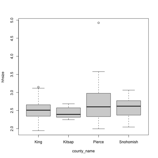
Say we want to look at the distribution of the average household sizes by counties. First, create a column for household size:

lu$hhsize <- lu$population/lu$households
head(lu[order(lu$hhsize),])

    city_id households   population  employment    city_name county_id
9         9     505387 982390.65316 871244.0433      Seattle        33
52       52        112    220.23109     68.0121    Skykomish        33
76       77       6894  13754.30315  13042.9198   Gig Harbor        53
135     136       1722   3520.86640    130.6559 Woodway MUGA        61
81       82        876   1810.73834    650.8074       Ruston        53
154     163         24     50.57888      0.0000      Roy PAA        53
    county_name   hhsize
9          King 1.943838
52         King 1.966349
76       Pierce 1.995112
135   Snohomish 2.044638
81       Pierce 2.067053
154      Pierce 2.107453

tail(lu[order(lu$hhsize),])

    city_id households  population  employment         city_name county_id
148     157        204   663.70020  7856.67975      Frederickson        53
152     161          4    13.21500    11.51667       Pacific PAA        53
74       75       4250 14641.94521 19597.32941              JBLM        53
143     152          6    21.44813     0.00000     Carbonado PAA        53
155     164         10    49.25578     0.00000 South Prairie PAA        53
133     134          0     0.00000  8332.60705  PAINE FIELD AREA        61
    county_name   hhsize
148      Pierce 3.253432
152      Pierce 3.303750
74       Pierce 3.445164
143      Pierce 3.574689
155      Pierce 4.925578
133   Snohomish      NaN

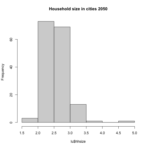
Second, create a histogram for all cities, and a box plot by counties:

hist(lu$hhsize, main = "Household size in cities 2050")

boxplot(hhsize ~ county_name, lu)

Saving plots

You can save a plot from within RStudio using the ‘Export’ button in the ‘Plot’ window. This will give you the option of saving as a .pdf or as .png, .jpg or other image formats.

Sometimes you will want to save plots without creating them in the ‘Plot’ window first. Perhaps you want to make a pdf document with multiple pages: each one a different plot, for example. Or perhaps you’re looping through multiple subsets of a file, plotting data from each subset, and you want to save each plot, but obviously can’t stop the loop to click ‘Export’ for each one.

In this case you can use a more flexible approach. The function pdf creates a new pdf device. You can control the size and resolution using the arguments to this function.

pdf("myplot.pdf", width=12, height=4)
par(mfrow=c(1,2)) # creates space for two graph panels in one row
hist(lu$hhsize)
boxplot(hhsize ~ county_name, lu)
# You then have to make sure to turn off the pdf device!
dev.off()

Open up this document and have a look.

The commands jpeg, png etc. are used similarly to produce documents in different formats.