Script Results
Suzanne Childress
1/8/2021
This shows the results of running all the steps of the class.
library(dplyr)## Warning: package 'dplyr' was built under R version 3.6.3##
## Attaching package: 'dplyr'## The following objects are masked from 'package:stats':
##
## filter, lag## The following objects are masked from 'package:base':
##
## intersect, setdiff, setequal, unionlibrary(stringr)
library(tidyr)## Warning: package 'tidyr' was built under R version 3.6.3library(ggplot2)## Warning: package 'ggplot2' was built under R version 3.6.3#### Restaurant Inspection Data ####
restaurant_file<-'C:/Users/SChildress/Documents/GitHub/intro-dplyr/data/king_county_restaurant_inspections.csv'
rest_df<-read.csv(restaurant_file, fileEncoding = 'UTF-8-BOM')
# find the dimensions of the data frame
dim(rest_df)## [1] 267167 15#look at the first five rows
head(rest_df)## OBJECTID FEATURE_ID NAME PROGRAM_IDENTIFIER
## 1 1 1 ARAMARK @ CONVENTION PLACE FLEX B
## 2 2 2 ARAMARK @ CONVENTION PLACE FLEX B
## 3 3 3 ARAMARK @ CONVENTION PLACE FLEX B
## 4 4 4 ARAMARK @ CONVENTION PLACE FLEX B
## 5 5 5 ARAMARK @ CONVENTION PLACE FLEX B
## 6 6 6 A & B CAFE A & B CAFE
## SEAT_CAP RISK ZIPCODE CITY DATE_INSPECTION
## 1 Seating 13-50 II 98101 Seattle 2017/10/27 00:00:00+00
## 2 Seating 13-50 II 98101 Seattle 2018/09/24 00:00:00+00
## 3 Seating 13-50 II 98101 Seattle 2016/08/30 00:00:00+00
## 4 Seating 13-50 II 98101 Seattle 2019/04/19 00:00:00+00
## 5 Seating 13-50 II 98101 Seattle 2018/04/17 00:00:00+00
## 6 Seating 13-50 III 98104 Seattle 2015/11/04 00:00:00+00
## TYPE_INSPECTION SCORE_INSPECTION RESULT_INSPECTION
## 1 Routine Inspection/Field Review 0 Satisfactory
## 2 Consultation/Education - Field 0 Complete
## 3 Consultation/Education - Field 0 Complete
## 4 Routine Inspection/Field Review 0 Satisfactory
## 5 Routine Inspection/Field Review 0 Satisfactory
## 6 Routine Inspection/Field Review 90 Unsatisfactory
## VIOLATIONTYPE
## 1
## 2
## 3
## 4
## 5
## 6 RED
## VIOLATIONDESCR
## 1
## 2
## 3
## 4
## 5
## 6 1400 - Raw meats below and away from ready to eat food; species separated
## VIOLATIONPOINTS
## 1 NA
## 2 NA
## 3 NA
## 4 NA
## 5 NA
## 6 5#what are the column names
colnames(rest_df)## [1] "OBJECTID" "FEATURE_ID" "NAME"
## [4] "PROGRAM_IDENTIFIER" "SEAT_CAP" "RISK"
## [7] "ZIPCODE" "CITY" "DATE_INSPECTION"
## [10] "TYPE_INSPECTION" "SCORE_INSPECTION" "RESULT_INSPECTION"
## [13] "VIOLATIONTYPE" "VIOLATIONDESCR" "VIOLATIONPOINTS"glimpse(rest_df)## Rows: 267,167
## Columns: 15
## $ OBJECTID <int> 1, 2, 3, 4, 5, 6, 7, 8, 9, 10, 11, 12, 13, ...
## $ FEATURE_ID <int> 1, 2, 3, 4, 5, 6, 7, 8, 9, 10, 11, 12, 13, ...
## $ NAME <fct> ARAMARK @ CONVENTION PLACE, ARAMARK @ CON...
## $ PROGRAM_IDENTIFIER <fct> FLEX B, FLEX B, FLEX B, FLEX B, FLEX B, A &...
## $ SEAT_CAP <fct> Seating 13-50, Seating 13-50, Seating 13-50...
## $ RISK <fct> II, II, II, II, II, III, III, III, III, III...
## $ ZIPCODE <int> 98101, 98101, 98101, 98101, 98101, 98104, 9...
## $ CITY <fct> Seattle, Seattle, Seattle, Seattle, Seattle...
## $ DATE_INSPECTION <fct> 2017/10/27 00:00:00+00, 2018/09/24 00:00:00...
## $ TYPE_INSPECTION <fct> Routine Inspection/Field Review, Consultati...
## $ SCORE_INSPECTION <int> 0, 0, 0, 0, 0, 90, 90, 90, 90, 90, 90, 90, ...
## $ RESULT_INSPECTION <fct> Satisfactory, Complete, Complete, Satisfact...
## $ VIOLATIONTYPE <fct> , , , , , RED, RED, RED, RED, BLUE, BLUE, B...
## $ VIOLATIONDESCR <fct> "", "", "", "", "", "1400 - Raw meats below...
## $ VIOLATIONPOINTS <int> NA, NA, NA, NA, NA, 5, 25, 25, 15, 5, 5, 5,...#### Basic dplyr verbs ####
# mutate() adds new variables that are functions of existing variables
# I'm going to add a new variable which is the year.
# Notice how I am using a %>% to use the mutate function on the rest_df.
rest_df <- rest_df %>% mutate('SEATTLE'= if_else(CITY=='Seattle', 'Seattle', 'Not Seattle'))
# select() picks variables based on their names.
less_columns_df <- rest_df %>% select('NAME', 'SEAT_CAP', 'VIOLATIONTYPE')
head(less_columns_df)## NAME SEAT_CAP VIOLATIONTYPE
## 1 ARAMARK @ CONVENTION PLACE Seating 13-50
## 2 ARAMARK @ CONVENTION PLACE Seating 13-50
## 3 ARAMARK @ CONVENTION PLACE Seating 13-50
## 4 ARAMARK @ CONVENTION PLACE Seating 13-50
## 5 ARAMARK @ CONVENTION PLACE Seating 13-50
## 6 A & B CAFE Seating 13-50 RED# filter() picks cases based on their values.
biz_df <- rest_df %>% dplyr::filter(str_detect(NAME, 'BIZ'))
bizzaro_df <- rest_df %>% dplyr::filter(str_detect(NAME, 'BIZZARRO'))
head(bizzaro_df)## OBJECTID FEATURE_ID NAME PROGRAM_IDENTIFIER
## 1 23407 23475 BIZZARRO ITALIAN CAFE BIZZARRO ITALIAN CAFE
## 2 23408 23476 BIZZARRO ITALIAN CAFE BIZZARRO ITALIAN CAFE
## 3 23409 23477 BIZZARRO ITALIAN CAFE BIZZARRO ITALIAN CAFE
## 4 23410 23478 BIZZARRO ITALIAN CAFE BIZZARRO ITALIAN CAFE
## 5 23411 23479 BIZZARRO ITALIAN CAFE BIZZARRO ITALIAN CAFE
## 6 23412 23480 BIZZARRO ITALIAN CAFE BIZZARRO ITALIAN CAFE
## SEAT_CAP RISK ZIPCODE CITY DATE_INSPECTION
## 1 Seating 13-50 III 98103 Seattle 2019/12/19 00:00:00+00
## 2 Seating 13-50 III 98103 Seattle 2018/12/14 00:00:00+00
## 3 Seating 13-50 III 98103 Seattle 2009/12/10 00:00:00+00
## 4 Seating 13-50 III 98103 Seattle 2009/12/10 00:00:00+00
## 5 Seating 13-50 III 98103 Seattle 2009/12/10 00:00:00+00
## 6 Seating 13-50 III 98103 Seattle 2017/12/07 00:00:00+00
## TYPE_INSPECTION SCORE_INSPECTION RESULT_INSPECTION
## 1 Routine Inspection/Field Review 0 Satisfactory
## 2 Consultation/Education - Field 0 Complete
## 3 Routine Inspection/Field Review 40 Unsatisfactory
## 4 Routine Inspection/Field Review 40 Unsatisfactory
## 5 Routine Inspection/Field Review 40 Unsatisfactory
## 6 Routine Inspection/Field Review 25 Unsatisfactory
## VIOLATIONTYPE
## 1
## 2
## 3 RED
## 4 RED
## 5 RED
## 6 RED
## VIOLATIONDESCR
## 1
## 2
## 3 1200 - Proper shellfish identification; proper parasit...
## 4 0200 - Food Worker Cards current for all food...
## 5 1600 - Proper cooling procedure
## 6 0500 - Proper barriers used to prevent bare hand contact with ready to eat foods.
## VIOLATIONPOINTS SEATTLE
## 1 NA Seattle
## 2 NA Seattle
## 3 5 Seattle
## 4 5 Seattle
## 5 30 Seattle
## 6 25 Seattle# you can stack the two operations together; like nesting a function
less_col_biz <- rest_df %>% select('NAME', 'VIOLATIONTYPE', 'VIOLATIONDESCR') %>% dplyr::filter(str_detect(NAME, 'BIZZARRO'))
head(less_col_biz)## NAME VIOLATIONTYPE
## 1 BIZZARRO ITALIAN CAFE
## 2 BIZZARRO ITALIAN CAFE
## 3 BIZZARRO ITALIAN CAFE RED
## 4 BIZZARRO ITALIAN CAFE RED
## 5 BIZZARRO ITALIAN CAFE RED
## 6 BIZZARRO ITALIAN CAFE RED
## VIOLATIONDESCR
## 1
## 2
## 3 1200 - Proper shellfish identification; proper parasit...
## 4 0200 - Food Worker Cards current for all food...
## 5 1600 - Proper cooling procedure
## 6 0500 - Proper barriers used to prevent bare hand contact with ready to eat foods.# arrange() changes the ordering of the rows.
# the default is ascending order, if you want descending use: desc
ordered_df <- bizzaro_df%>% arrange(desc(SCORE_INSPECTION))
head(ordered_df)## OBJECTID FEATURE_ID NAME PROGRAM_IDENTIFIER
## 1 23409 23477 BIZZARRO ITALIAN CAFE BIZZARRO ITALIAN CAFE
## 2 23410 23478 BIZZARRO ITALIAN CAFE BIZZARRO ITALIAN CAFE
## 3 23411 23479 BIZZARRO ITALIAN CAFE BIZZARRO ITALIAN CAFE
## 4 23418 23486 BIZZARRO ITALIAN CAFE BIZZARRO ITALIAN CAFE
## 5 23419 23487 BIZZARRO ITALIAN CAFE BIZZARRO ITALIAN CAFE
## 6 23426 23494 BIZZARRO ITALIAN CAFE BIZZARRO ITALIAN CAFE
## SEAT_CAP RISK ZIPCODE CITY DATE_INSPECTION
## 1 Seating 13-50 III 98103 Seattle 2009/12/10 00:00:00+00
## 2 Seating 13-50 III 98103 Seattle 2009/12/10 00:00:00+00
## 3 Seating 13-50 III 98103 Seattle 2009/12/10 00:00:00+00
## 4 Seating 13-50 III 98103 Seattle 2014/09/30 00:00:00+00
## 5 Seating 13-50 III 98103 Seattle 2014/09/30 00:00:00+00
## 6 Seating 13-50 III 98103 Seattle 2015/07/28 00:00:00+00
## TYPE_INSPECTION SCORE_INSPECTION RESULT_INSPECTION
## 1 Routine Inspection/Field Review 40 Unsatisfactory
## 2 Routine Inspection/Field Review 40 Unsatisfactory
## 3 Routine Inspection/Field Review 40 Unsatisfactory
## 4 Routine Inspection/Field Review 35 Unsatisfactory
## 5 Routine Inspection/Field Review 35 Unsatisfactory
## 6 Routine Inspection/Field Review 30 Unsatisfactory
## VIOLATIONTYPE
## 1 RED
## 2 RED
## 3 RED
## 4 RED
## 5 RED
## 6 RED
## VIOLATIONDESCR
## 1 1200 - Proper shellfish identification; proper parasit...
## 2 0200 - Food Worker Cards current for all food...
## 3 1600 - Proper cooling procedure
## 4 1900 - No room temperature storage; proper use of time...
## 5 2110 - Proper cold holding temperatures (greater than 45 degrees F)
## 6 1600 - Proper cooling procedure
## VIOLATIONPOINTS SEATTLE
## 1 5 Seattle
## 2 5 Seattle
## 3 30 Seattle
## 4 25 Seattle
## 5 10 Seattle
## 6 25 Seattle#### Group by and Summarize ####
# Let's count the records in our data.
rest_df_count <- rest_df %>% count()
rest_df_count## n
## 1 267167# Now let's count the number of observations for each restaurant.
rest_df_count2 <- rest_df %>% count(NAME)
head(rest_df_count2)## NAME n
## 1 A-CHAU CAFE 65
## 2 A-PIZZA MART 53
## 3 A-STREET BIG FOOT JAVA 12
## 4 A & B CAFE 48
## 5 A & S PETROLEUM LCC 27
## 6 A BAO TIME LLC DBA Phorale 35rest_df_count_sort<-rest_df %>% count(NAME,sort=TRUE)
head(rest_df_count_sort)## NAME n
## 1 T-MOBILE PARK 1977
## 2 TACO TIME 1160
## 3 SUBWAY 1049
## 4 WHOLE FOODS MARKET 972
## 5 PCC COMMUNITY MARKETS 832
## 6 STARBUCKS COFFEE 736#### Data Wrangling ####
# I want to find out the unique values of the type of inspections
unique(rest_df$TYPE_INSPECTION)## [1] Routine Inspection/Field Review Consultation/Education - Field
## [3] Return Inspection
## 3 Levels: Consultation/Education - Field ... Routine Inspection/Field Reviewglimpse(rest_df)## Rows: 267,167
## Columns: 16
## $ OBJECTID <int> 1, 2, 3, 4, 5, 6, 7, 8, 9, 10, 11, 12, 13, ...
## $ FEATURE_ID <int> 1, 2, 3, 4, 5, 6, 7, 8, 9, 10, 11, 12, 13, ...
## $ NAME <fct> ARAMARK @ CONVENTION PLACE, ARAMARK @ CON...
## $ PROGRAM_IDENTIFIER <fct> FLEX B, FLEX B, FLEX B, FLEX B, FLEX B, A &...
## $ SEAT_CAP <fct> Seating 13-50, Seating 13-50, Seating 13-50...
## $ RISK <fct> II, II, II, II, II, III, III, III, III, III...
## $ ZIPCODE <int> 98101, 98101, 98101, 98101, 98101, 98104, 9...
## $ CITY <fct> Seattle, Seattle, Seattle, Seattle, Seattle...
## $ DATE_INSPECTION <fct> 2017/10/27 00:00:00+00, 2018/09/24 00:00:00...
## $ TYPE_INSPECTION <fct> Routine Inspection/Field Review, Consultati...
## $ SCORE_INSPECTION <int> 0, 0, 0, 0, 0, 90, 90, 90, 90, 90, 90, 90, ...
## $ RESULT_INSPECTION <fct> Satisfactory, Complete, Complete, Satisfact...
## $ VIOLATIONTYPE <fct> , , , , , RED, RED, RED, RED, BLUE, BLUE, B...
## $ VIOLATIONDESCR <fct> "", "", "", "", "", "1400 - Raw meats below...
## $ VIOLATIONPOINTS <int> NA, NA, NA, NA, NA, 5, 25, 25, 15, 5, 5, 5,...
## $ SEATTLE <chr> "Seattle", "Seattle", "Seattle", "Seattle",...# The DATE_INSPECTION FIELD is a factor, but we want it to be a date so we filter on it.
rest_df <- rest_df %>% mutate(DATE_INSP_FORMAT=as.Date(word(as.character(DATE_INSPECTION), 1)))
#let's check to see that now the DATE_INSP_FORMAT field looks like a date and is okay
glimpse(rest_df)## Rows: 267,167
## Columns: 17
## $ OBJECTID <int> 1, 2, 3, 4, 5, 6, 7, 8, 9, 10, 11, 12, 13, ...
## $ FEATURE_ID <int> 1, 2, 3, 4, 5, 6, 7, 8, 9, 10, 11, 12, 13, ...
## $ NAME <fct> ARAMARK @ CONVENTION PLACE, ARAMARK @ CON...
## $ PROGRAM_IDENTIFIER <fct> FLEX B, FLEX B, FLEX B, FLEX B, FLEX B, A &...
## $ SEAT_CAP <fct> Seating 13-50, Seating 13-50, Seating 13-50...
## $ RISK <fct> II, II, II, II, II, III, III, III, III, III...
## $ ZIPCODE <int> 98101, 98101, 98101, 98101, 98101, 98104, 9...
## $ CITY <fct> Seattle, Seattle, Seattle, Seattle, Seattle...
## $ DATE_INSPECTION <fct> 2017/10/27 00:00:00+00, 2018/09/24 00:00:00...
## $ TYPE_INSPECTION <fct> Routine Inspection/Field Review, Consultati...
## $ SCORE_INSPECTION <int> 0, 0, 0, 0, 0, 90, 90, 90, 90, 90, 90, 90, ...
## $ RESULT_INSPECTION <fct> Satisfactory, Complete, Complete, Satisfact...
## $ VIOLATIONTYPE <fct> , , , , , RED, RED, RED, RED, BLUE, BLUE, B...
## $ VIOLATIONDESCR <fct> "", "", "", "", "", "1400 - Raw meats below...
## $ VIOLATIONPOINTS <int> NA, NA, NA, NA, NA, 5, 25, 25, 15, 5, 5, 5,...
## $ SEATTLE <chr> "Seattle", "Seattle", "Seattle", "Seattle",...
## $ DATE_INSP_FORMAT <date> 2017-10-27, 2018-09-24, 2016-08-30, 2019-0...rest_df<-rest_df %>% dplyr::mutate(VIOLATIONPOINTS = replace_na(VIOLATIONPOINTS, 0))
rest_df_filtered <- rest_df %>% filter(TYPE_INSPECTION=='Routine Inspection/Field Review') %>%
group_by(NAME) %>%
filter(DATE_INSP_FORMAT == max(DATE_INSP_FORMAT)) %>%
slice(which.max(VIOLATIONPOINTS))
#### Playing with the Data ####
glimpse(rest_df_filtered)## Rows: 8,961
## Columns: 17
## Groups: NAME [8,961]
## $ OBJECTID <int> 911, 8306, 11138, 26, 77, 13518, 82, 92, 11...
## $ FEATURE_ID <int> 914, 8336, 11173, 26, 77, 13562, 82, 92, 11...
## $ NAME <fct> "A-CHAU CAFE", "A-PIZZA MART", "A-STREET BI...
## $ PROGRAM_IDENTIFIER <fct> "A-CHAU CAFE", "A-PIZZA MART", "A-STREET BI...
## $ SEAT_CAP <fct> Seating 13-50, Seating 0-12, Seating 0-12, ...
## $ RISK <fct> III, III, I, III, III, III, III, III, III, ...
## $ ZIPCODE <int> 98118, 98126, 98002, 98104, 98028, 98134, 9...
## $ CITY <fct> Seattle, Seattle, Auburn, Seattle, Kenmore,...
## $ DATE_INSPECTION <fct> 2020/01/21 00:00:00+00, 2020/01/16 00:00:00...
## $ TYPE_INSPECTION <fct> Routine Inspection/Field Review, Routine In...
## $ SCORE_INSPECTION <int> 0, 0, 8, 15, 18, 50, 12, 10, 0, 30, 5, 60, ...
## $ RESULT_INSPECTION <fct> Satisfactory, Satisfactory, Satisfactory, U...
## $ VIOLATIONTYPE <fct> , , BLUE, RED, RED, RED, RED, RED, , RED, B...
## $ VIOLATIONDESCR <fct> "", "", "3400 - Wiping cloths properly used...
## $ VIOLATIONPOINTS <dbl> 0, 0, 5, 5, 10, 25, 5, 5, 0, 25, 5, 25, 25,...
## $ SEATTLE <chr> "Seattle", "Seattle", "Not Seattle", "Seatt...
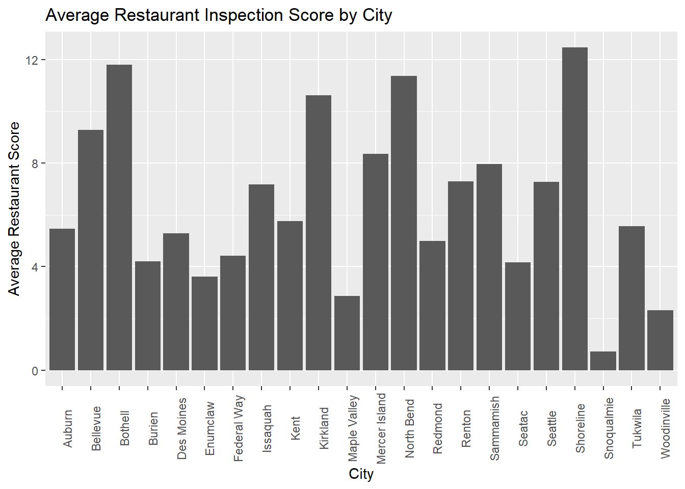
## $ DATE_INSP_FORMAT <date> 2020-01-21, 2020-01-16, 2019-10-22, 2019-0...#How do the inspection score vary by city?
# Average and Max Score by City
score_by_city<-rest_df_filtered %>% group_by(CITY) %>% summarize(avg_score= mean(SCORE_INSPECTION),
max_score = max(SCORE_INSPECTION),
n_rests = n())## `summarise()` ungrouping output (override with `.groups` argument)score_by_city## # A tibble: 51 x 4
## CITY avg_score max_score n_rests
## <fct> <dbl> <int> <int>
## 1 (None) 5 5 1
## 2 Algona 2.67 16 6
## 3 Auburn 5.46 77 265
## 4 Baring 0 0 1
## 5 Bellevue 9.29 100 610
## 6 Black Diamond 2.74 23 19
## 7 Bothell 11.8 70 83
## 8 Burien 4.21 50 148
## 9 Carnation 0.5 5 26
## 10 Clyde Hill 3.25 13 4
## # ... with 41 more rows# some of the cities have very few restaurants; let's remove those
score_city_sufficient <- score_by_city %>% filter(n_rests>50)
#dplyr works great with ggplot to make plots.
ggplot(data=score_city_sufficient, aes(x=CITY, y=avg_score)) +
geom_bar(stat="identity")+theme(axis.text.x = element_text(angle = 90))+
ggtitle("Average Restaurant Inspection Score by City") +
xlab("City") + ylab("Average Restaurant Score")
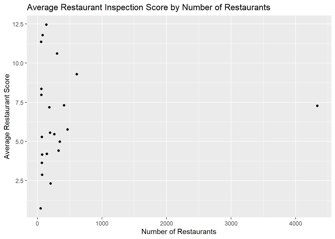
# does the average score just correlate with number of restaurants?
ggplot(data=score_city_sufficient, aes(x=n_rests, y=avg_score)) +
  geom_point()+ggtitle("Average Restaurant Inspection Score by Number of Restaurants") +
  xlab("Number of Restaurants") + ylab("Average Restaurant Score")
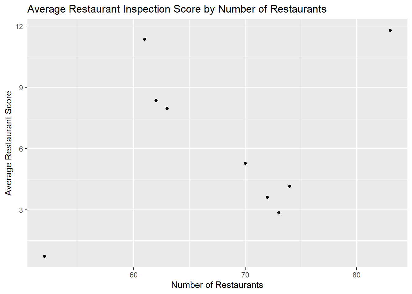
# Seattle throws everything off
score_city_sufficient_not_too_many <- score_city_sufficient %>% filter(n_rests<100)
ggplot(data=score_city_sufficient_not_too_many, aes(x=n_rests, y=avg_score)) +
  geom_point()+ggtitle("Average Restaurant Inspection Score by Number of Restaurants") +
  xlab("Number of Restaurants") + ylab("Average Restaurant Score")
# What is the info on the restaurant with the worst score by city?

worst_by_city<-rest_df_filtered %>% group_by(CITY) %>% top_n(1, SCORE_INSPECTION)

worst_by_city
## # A tibble: 60 x 17
## # Groups: CITY [51]
## OBJECTID FEATURE_ID NAME PROGRAM_IDENTIF~ SEAT_CAP RISK ZIPCODE CITY
## <int> <int> <fct> <fct> <fct> <fct> <int> <fct>
## 1 6675 6701 AMBA~ AMBAKITY COCINA~ Mobile ~ III 98002 Aubu~
## 2 9442 9472 ARCH~ ARCHIE'S MEXICA~ Seating~ III 98148 Norm~
## 3 10794 10829 ASIA~ ASIAN PLANET FO~ Meat/Se~ III 98030 Kent
## 4 19610 19667 BEEC~ BEECHER'S CHEES~ Seating~ III 98158 Seat~
## 5 21729 21787 BEST~ BEST OF BOTH WO~ Mobile ~ III 98296 Snoh~
## 6 22364 22426 BIG ~ BIG AIR BAR-B-Q~ Seating~ III 98045 Snoq~
## 7 36490 36636 CASA~ CASA BONITA Seating~ III 98070 Vash~
## 8 36540 36686 CASA~ CASA DURANGO Seating~ III 98148 Norm~
## 9 37437 37588 CATH~ CATHOUSE KC422 ~ Mobile ~ III 98290 Snoh~
## 10 46096 46269 COCO~ COCO JOE'S Seating~ III 98001 Algo~
## # ... with 50 more rows, and 9 more variables: DATE_INSPECTION <fct>,
## # TYPE_INSPECTION <fct>, SCORE_INSPECTION <int>,
## # RESULT_INSPECTION <fct>, VIOLATIONTYPE <fct>, VIOLATIONDESCR <fct>,
## # VIOLATIONPOINTS <dbl>, SEATTLE <chr>, DATE_INSP_FORMAT <date># What was the data on the restaurant I liked?
bizzaro_df_filtered <- rest_df_filtered %>% dplyr::filter(str_detect(NAME, 'BIZZARRO'))
bizzaro_df_filtered## # A tibble: 1 x 17
## # Groups: NAME [1]
## OBJECTID FEATURE_ID NAME PROGRAM_IDENTIF~ SEAT_CAP RISK ZIPCODE CITY
## <int> <int> <fct> <fct> <fct> <fct> <int> <fct>
## 1 23407 23475 BIZZ~ BIZZARRO ITALIA~ Seating~ III 98103 Seat~
## # ... with 9 more variables: DATE_INSPECTION <fct>, TYPE_INSPECTION <fct>,
## # SCORE_INSPECTION <int>, RESULT_INSPECTION <fct>, VIOLATIONTYPE <fct>,
## # VIOLATIONDESCR <fct>, VIOLATIONPOINTS <dbl>, SEATTLE <chr>,
## # DATE_INSP_FORMAT <date>############### Exercises ################
# 1. Find your a restaurant of your choice and get the latest data.
# 2. Go back to the big dataset and find the worst violation of a restaurant you want.
# 3. Make a table that shows grouped RISK category and the average and max SCORE_INSPECTION
# 4. Make a table that shows grouped SEAT_CAP and the average and max SCORE_INSPECTION
# 5. Find out which VIOLATIONDESCR is associated with the the highest SCORE_INSPECTION
# 6. Make a barplot that shows the maximum inspection score by city.